Bye bye, academia.edu and ResearchGate – hello PsyArXiv!

There’s lots of stuff I should be doing right now (most imminently, preparing syllabi), but I’ve been meaning to do this for a while. Specifically: I want for-profit companies academia.edu and ResearchGate.com out of my life.

Luckily, psychology now has a robust, not-for-profit alternative allowing us to share both pre-prints and post-prints*, a service called PsyArXiv. Here are seven reasons I hope you’ll join me now (or even slowly, migrating your work over time):

    1. Open Access: You want your work to be freely available, even to scholars who don’t  have library access and the general public. For most psychology journals, you don’t have to pay an OA fee to make your (un-typeset) work freely available to all.
    2. Higher Citation Rates: Work that is made accessible tends to be accessed and used more. PsyArXiv tracks your download counts, and I can confirm that it is weirdly satisfying to see those numbers tick up over time.
    3. Indexed by Google Scholar: When people search for your work on Google Scholar, they’ll get directed to your freely accessible pre-print.
    4. Link to Published Work: You can assign DOIs to your pre-prints on OSF, and if applicable you can associate the pre-print with the DOI of a published paper.
    5. Version Control: With preprints on PsyArXiv, you can easily update your work to the latest version, while simply keeping track of earlier versions. Readers get the latest version – perfect for incorporating corrections and updates.
    6. Archive and Preserve: PsyArXiv is hosted by the Open Science Framework, and content there is backed by a $250,000 endowment to ensure your work is stably hosted. Storage on PsyArXiv is designed to be more reliable and longer lasting than storage on your personal website or computer.
    7. Supported and Maintained by the Research Community: We researchers already cede too much control of our work to for-profit publishers – why give for-profit entities any leg up at all in the preprint space? This one is easy: I’ll choose instead to support the site that is maintained by my peers**.

You can check out this PsyArXiv blog  post (and the others) to learn more about the preprint initiative.

So you’re on board? Here’s how to do the same:

  1. Post your author formatted copies of your papers on PsyArXiv***. You can check SHERPA/RoMEO to make sure it is OK to post  your own copies of your published or accepted papers (it is for most psych journals).
  2. Delete any .pdfs you are hosting on academia.edu or ResearchGate.com. If you have co-authors who have posted copies of your work, consider asking them to take those copies down. (Here’s how I did so.)
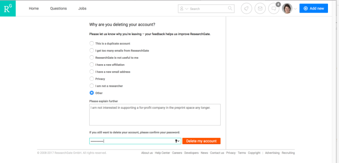
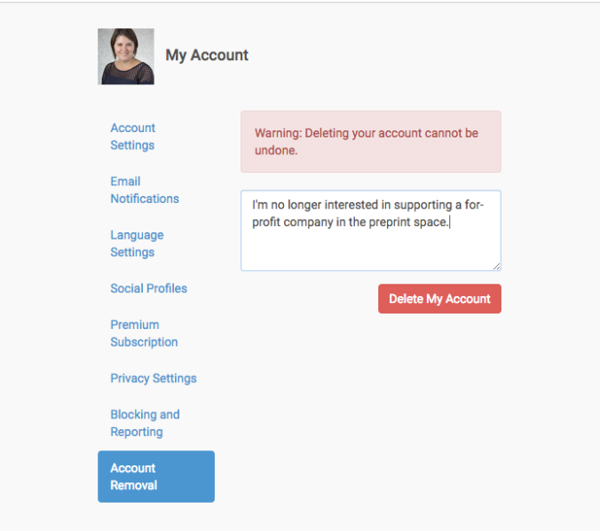
  3. Delete your academia.edu and ResearchGate.com accounts. It’s in the settings area for both sites. Here’s my screen grabs from doing so:


The last step is to tell your colleagues and share on social media. I bet if we work together we can give for-profit preprint hosts the boot. Will you join me?


* Terminology- To me a pre-print is a “working paper” that has not yet been accepted for publication, whereas a post-print is a published paper that you’re sharing on a pre-print server like PsyArXiv. Some people use working paper or draft paper to correspond to the pre-acceptance stage of a paper, pre-print to mean the “Online Advance” copy, and post-print to mean the final formatted paper after it is in a particular issue of a journal. I think it’s fair to say that not everyone uses these terms super clearly or consistently, myself included. [back]

** Shameless promotion – PsyArXiv was developed at SIPS 2016 and continues to be maintained by a board, chaired by the awesome Ben Brown. +1 for community-driven improvements! [back]

***One thing to consider is how to license your work when you post on PsyArXiv. CC0 and CC-BY are two licensing options that allow greatest re-use of your work (e.g., in educational settings, in future works like edited collections). You can read more here. Thanks to Chris Hartgerink for raising this key point! [back]

Dr. Wide Net has a lower False Discovery Rate than Dr. Power

Will Gervais just posted a really, really cool simulation showing differences in the number of findings discovered by Dr. Power (who runs 100 person per condition studies, all day everyday) and Dr. Wide Net (who runs 25 person per condition pilot studies and follows up on promising – aka statistically significant – ideas). Both researchers have access to a limited number (4,000) of participants in a given year. The question is, which strategy is better for netting creative new ideas?

Luckily for me, Will shared his code. The code is amazing, and Will is modest. It was easy to modify and add a few pieces to find out a few things I wanted to know. Specifically, Will presents the rate of “findings” (aka true positives) that each approach yields. But what about false positives? Missed effects (aka false negatives)? Correct rejections? Are there any differences for these other findings for Dr. Power vs. Dr. Wide Net? My results are below – as figures instead of tables, sorry Will!

numbs_findings_line

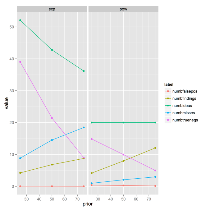
Dr. Power is on the right, and Dr. Wide Net is on the left. I ran the simulation at 3 different prior levels (.25, .50, .75), because I’m even lazier than Will claims to be (he’s obviously not, given this awesome sim). The green line represents the total number of ideas tested (I replicate Will’s finding that for Dr. Wide Net, the number of ideas tested goes down as the prior goes up, whereas for Dr. Power, the number of ideas tested is a direct function of n/cell and total N).

The yellow-y line is the number of true positives (“findings”) identified. Just as Will found, I find that as the prior goes up, Dr. Power finds more findings. (Note that my simulation is done with the alpha for Dr. Wide Net’s pilot studies set at .10, so the same as Will’s Table 2).

The purple line is the number of findings that represent true negatives (i.e., no effect exists, and the test returns non-significant). These go down as the prior goes up, definitionally.

The blue line represents the number of misses – true effects that go undetected. Dr. Wide Net has a ton of these! Dr. Power barely misses out on any effects. This makes sense, because Dr. Wide Net is sacrificing power for the ability to test many ideas. Lower power means that there will be more missed true effects, by definition. (However, for both Drs., misses increase as the prior increases. I don’t actually know why this is. Why should power decrease as the prior increases? Readers?)

Now here’s where it gets really strange. It’s almost imperceptible in the graph above, but the rate of false positives is higher for Dr. Power than it is for Dr. Wide Net. Neither doctor has a particularly high false positive rate, but Dr. Power’s rate is higher. What’s going on? My hunch is that Dr. Wide Net’s filtering of the effects she studies (via pilot testing) is helping to lower the overall false positive rate of her studies.

Let’s look at these results another way:

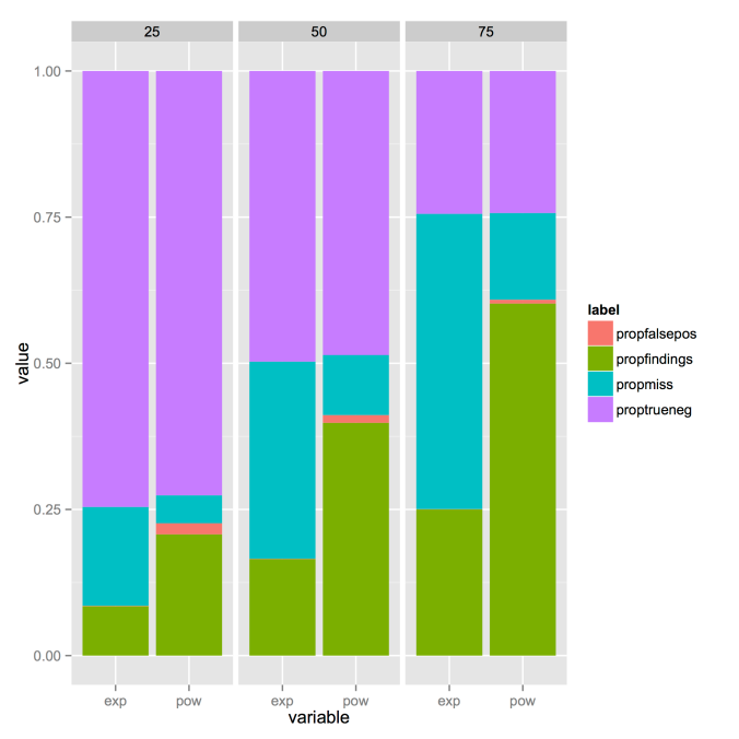
props_findings_stackedbar

Here we can clearly see that the rate of false positive studies is more perceptible for Dr. Power than Dr. Wide Net (this figure shows the percentage of studies done that yield a particular result). As we know, Dr. Wide Net does way, way more studies.

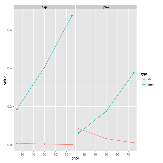
Another way to think about this is as the False Discovery Rate, or the proportion of statistically significant findings that are false positives. We can also consider the False Omission Rate, the proportion of non-significant findings that are missed (false negatives). Here’s a graph:

fdr_fomr

Dr. Power does have a higher false discovery rate (but the FDR decreases as the prior increases). Dr. Wide Net’s false discovery rate is almost zero. So this is a little weird, because it almost seems like a win for Dr. Wide Net.

BUT – and there’s always a but!

Dr. Wide Net’s False Omission Rate is off the charts. With a 50-50 prior, about 40% of Dr. Wide Net’s non-significant results are actually real effects. By contrast, with the same prior, Dr. Power has only about 18% non-significant results that are actually real effects. When we take this finding into account together with efficiency (again, Dr. Wide Net has to do tons more studies than Dr. Power), I’m pretty sure the lower false discovery rate isn’t worth it.

My code (a slightly modified version of Will’s) is here. I welcome corrections and comments!


So You Want to Pre-Register a Study

SPSP 2016 has just wrapped up and with it another year of fantastic meetings and discussion. This year, I (together with Jordan Axt, Erica Baranski, and David Condon) hosted a professional development session on daily open science practices – little things you can do each day to make your work more open and reproducible. You can find all of our materials for the session here, but I wanted to elaborate on my portion of the session concerning pre-registration.

A person approached me after the session and told me the following:

“I want to give this pre-registration thing a try, but I don’t know where to start. How can I show an editor that my work is pre-registered?”

So here it is: a how-to guide to pre-registration. As I said at SPSP, there is not one perfect/only way to pre-register – scientists can choose to pre-register only locally (nothing online – just some documentation for themselves), privately (pre-registration plan posted online, but with closed access), or publicly (pre-registration plan posted online, in a registry, and free for all to see). The key ingredient across all of these approaches is that flexibility in analysis and design is constrained by pre-specifying the researcher’s plan (more on that in a bit). For now, let’s consider the options one-by-one.

1. Internal only pre-registration: Within-team (local) documentation of study design, planned hypothesis tests and analyses, planned exclusion rules, and so on, prior to data collection.

Pros: Pre-registration in any form helps you slow down and be more sure that your project can test the question you want it to. I would argue that the quality of science improves as a result. You have protection, even if only to yourself and your team, against over-interpreting an exploratory finding (by decreasing hindsight bias or reducing hypothesizing after the results are known, aka HARKing).

Cons: An editor or reviewer doesn’t have evidence, apart from your word, that the pre-registration actually happened. A scientist’s word is worth a lot, but when it comes to convincing a skeptic, you might have a tough time.

Options: Your imagination is the limit when it comes to thinking of ways to do internal documentation. You could go old-school and write long-hand in ink in a lab notebook. You could use Evernote or Google docs or some other kind of cloud based document storage. The key is that you make your notes to yourself (and perhaps your local team), and those notes don’t get edited later on. They are just a record of your plans. I should note that you would benefit from using a standard type of template (more on templates in a minute), if only so that you don’t forget to think through the most important factors in your study (trust me, forgetting happens to the best of us).

2. Private pre-registration: Same as internal only pre-registration, except you post the pre-registration privately to a repository. Private pre-registrations can be selectively shared with editors and reviewers, for the purposes of proving that a pre-registration occurred as specified.

Pros: You cannot be “scooped” – meaning your ideas stay private until such time as you later choose, but you can definitively prove that your (perhaps un-Orthodox) analysis was the plan all along.

Cons: You cannot attract collaborators, either. Others working in a similar area don’t know what you’re up to, and you might miss out on a valuable collaboration. For the field writ large, this isn’t a very attractive long term option, because we don’t get a record of abandoned projects either – studies that for whatever reason don’t make it past the data collection stage and into the published literature.

Options: For easy to do private pre-registration, you can’t beat aspredicted.org. One author on the team simply answers 9 questions about the planned project, and a .pdf of the pre-registration is generated. Pre-registrations can stay private indefinitely on aspredicted, but authors do have the option to generate a web link to share with editors/reviewers. Another option would be to use the Open Science Framework (osf.io). The OSF has a pre-registration function that researchers can choose to make private for up to 4 years (at which point, the pre-registration does become public).  The pre-registration function freezes the content of an OSF project so that a record of the project is preserved and no longer able to be edited. As an alternative to the pre-registration function, OSF timestamps all researcher activity on the site, and it allows researchers to keep their (non-registered) projects private indefinitely. This means that a researcher could post a document containing a pre-registration to their private project and use the OSF timestamping system to prove to an outside party when the pre-registration occurred, relative to when data were collected. The clunkiness of this system means that researchers who want to have indefinitely private pre-registrations will likely want to use aspredicted.org, or use OSF and accept that after the researcher-determined embargo period of up to 4 years, their pre-registrations will become public. Again, the public vs. private distinction has downstream consequences for the field, because public pre-registrations allow researchers to understand the magnitude of the file drawer problem in a given area of the literature.

3. Public pre-registration: Same as private pre-registration, except that researchers post their plans publicly on the web.

Pros: Fully open, complete with mega-credibility points. Your work is fully verifiable to an outside party. Outside parties can contact you and ask to collaborate. As a side note, we all have projects that are interesting and potentially fruitful, but that get left by the wayside due to lack of time or other constraints. To me, pre-registration (or really any form of transparent documentation) is a way of keeping track of these projects and letting others pick them up as the years go on (I have this fantasy that when a student joins my lab, I’ll be able to direct them to the documentation of an in-progress, but stalled, project, and they’ll just pick it right back up where the previous student faltered). So there are potential benefits of increased transparency and better record keeping beyond the type-I error control that proponents of pre-registration are so quick to note.

Cons: Scooping? I’m not sure this is a real concern, but insofar as people have anxiety about it, it needs to be addressed. If you make your whole train of logic/program of research fully transparent, there is always the risk that someone better/smarter/faster/stronger than you will swoop in and run off with the idea. To me, the potential for fruitful collaborations far outweighs the risk of scooping, and actually both are trumped by a third possibility, which is that all this documentation won’t attract much attention at all. In my own experience, a handful of people are interested, but mostly my work goes on as usual. Others have noted that public pre-registration actually could help you stake a claim on a project, insofar as you are able to demonstrate the temporal precedence of the idea relative to the alleged scoop-er. A final con is that there is a time cost to getting the study materials up to snuff for public consumption. However, as I noted before, the quality of the work likely increases, and the project is less likely to get shelved if a collaborator loses interest or there are other hiccups down the road. I’m a big fan of designing studies so that they are informative, null results or not, so that there is (ideally) no such thing as a “failed” study, and instead only limitations in our time, motivation, and fiscal resources to publish every (properly executed) study. Doing a good job of documentation on the front end of a project means that even if you never get around to publishing a boring/null/whatever result, a future meta-analyst could, with some ease, find your project and incorporate it into their work.

Options: The OSF is likely to be your best bet at this point, and although OSF is a powerful, flexible system, it is not the most user friendly for beginners. However, the opportunity cost of learning the system more than pays for itself down the road. Anna van’t Veer and Roger Giner-Sorolla have this nice step-by-step that explains how to create and pre-register a new project on OSF. The Center for Open Science pre-registration challenge also has a bunch of materials that will help you get started. And if you want to do the pre-registration challenge, and you’re an R user, you’ll definitely want to check out Frederick Aust’s prereg package for R.


Regardless of which option you choose to pursue, I would encourage you to think about using a template (either make your own or use someone else’s) so that you get all of the most important details of your project ironed out ahead of time. It will definitely happen that once you have your data in hand, you realize that you’ve forgotten to specify something important. That’s OK, and you ought to just honestly report such discrepancies and move on. Don’t let perfect be the enemy of done.

Templates:

  • Alison Ledgerwood’s internal pre-reg template
  • Sample aspredicted.org pre-reg form
  • Sample pre-reg challenge form (from Aust’s prereg R package)

Feedback, comments, and questions welcome! Leave a note on the post, write me on Twitter (@katiecorker), or shoot me an email (corkerk at kenyon dot edu).
When Study 1 & Study 2 Disagree: Practical Recommendations for Researchers

A friend posted a question to a group of research colleagues recently:

“Three weeks ago, I ran a 100 person two-condition study on Mturk. Result: t = 2.95, p = .004. Today I ran another 100 person two condition study on Mturk, using the identical measure. No differences in what came before that measure. Result? t = 0.13, p = .89.”

The friend was exasperated and didn’t know what to do – What are the best practices for how researchers should adjudicate conflicting study results like these? I wrote the friend a long response, but I realized that my advice might be of use to others too.

The group had several suggestions for courses of action. I list the options below and explain my preferred option.

  1. Drop the project. This is an unsatisfactory choice, because as we will see below, the first two studies were likely underpowered, so we’re risking missing out on a true effect by abandoning the research question too soon (i.e., we risk a Type II error).
  2. Report the significant study and ignore the non-significant one. Ok, no one actually recommended this choice. But I think this is what a mentor might have recommended back in the old days. We know now that file drawering the non-significant study substantially inflates the Type I error rate of the published literature, which would be dishonest and not cool.
  3. Look for a moderator. Perhaps the first study was run on a Tuesday, and the effect only shows up on Tuesday. Or perhaps, more interestingly, the first study had more women participants, and the effect is stronger for women participants. These post-hoc moderators could explain why the effect shows up in one study but not the other. However, there are an infinite number of these potential moderators, and we have no way of knowing for sure which one is actually responsible. The most likely explanation is simple sampling error.
  4. Meta-analyze and use the meta-analytic confidence interval to test significance of the effect. This is not a terrible choice, and in the absence of more resources to conduct further research, this is probably a researcher’s best bet. But ultimately, without additional data, we can’t be very confident whether Study 1 was a false positive or Study 2 was a false negative.
  5. Use the meta-analytic effect size estimate to determine the needed sample size for a third study with 80% power. This is my recommended, best practices, option for the reasons outlined in point 4. Note that this third study should not be viewed as a tiebreaker, but rather as a way to get a more precise estimate of the actual effect size in question.

What follows is a step-by-step guide using the R statistics software package to conduct the meta-analysis and estimate the number of participants needed for Study 3.

Step 0 – Download the compute.es, metafor, and pwr libraries if you don’t have them already. This step only needs to be completed once per computer. You’ll need to remove the # first.

#install.packages("compute.es", repos='http://cran.us.r-project.org')
#install.packages("metafor", repos='http://cran.us.r-project.org')
#install.packages("pwr", repos='http://cran.us.r-project.org')

Step 1 – Then load the packages:

library(compute.es)
library(metafor)
## Loading required package: Matrix
## Loading 'metafor' package (version 1.9-7). For an overview 
## and introduction to the package please type: help(metafor).
library(pwr)

Step 2 – Compute the effect sizes for your studies.

study1<-tes(t=2.95,n.1=50,n.2=50)
## Mean Differences ES: 
##  
##  d [ 95 %CI] = 0.59 [ 0.18 , 1 ] 
##   var(d) = 0.04 
##   p-value(d) = 0 
##   U3(d) = 72.24 % 
##   CLES(d) = 66.17 % 
##   Cliff's Delta = 0.32 
##  
##  g [ 95 %CI] = 0.59 [ 0.18 , 0.99 ] 
##   var(g) = 0.04 
##   p-value(g) = 0 
##   U3(g) = 72.09 % 
##   CLES(g) = 66.06 % 
##  
##  Correlation ES: 
##  
##  r [ 95 %CI] = 0.29 [ 0.09 , 0.46 ] 
##   var(r) = 0.01 
##   p-value(r) = 0 
##  
##  z [ 95 %CI] = 0.29 [ 0.09 , 0.5 ] 
##   var(z) = 0.01 
##   p-value(z) = 0 
##  
##  Odds Ratio ES: 
##  
##  OR [ 95 %CI] = 2.92 [ 1.4 , 6.08 ] 
##   p-value(OR) = 0 
##  
##  Log OR [ 95 %CI] = 1.07 [ 0.33 , 1.81 ] 
##   var(lOR) = 0.14 
##   p-value(Log OR) = 0 
##  
##  Other: 
##  
##  NNT = 4.98 
##  Total N = 100
study2<-tes(t=0.13,n.1=50,n.2=50)
## Mean Differences ES: 
##  
##  d [ 95 %CI] = 0.03 [ -0.37 , 0.42 ] 
##   var(d) = 0.04 
##   p-value(d) = 0.9 
##   U3(d) = 51.04 % 
##   CLES(d) = 50.73 % 
##   Cliff's Delta = 0.01 
##  
##  g [ 95 %CI] = 0.03 [ -0.37 , 0.42 ] 
##   var(g) = 0.04 
##   p-value(g) = 0.9 
##   U3(g) = 51.03 % 
##   CLES(g) = 50.73 % 
##  
##  Correlation ES: 
##  
##  r [ 95 %CI] = 0.01 [ -0.19 , 0.21 ] 
##   var(r) = 0.01 
##   p-value(r) = 0.9 
##  
##  z [ 95 %CI] = 0.01 [ -0.19 , 0.21 ] 
##   var(z) = 0.01 
##   p-value(z) = 0.9 
##  
##  Odds Ratio ES: 
##  
##  OR [ 95 %CI] = 1.05 [ 0.51 , 2.15 ] 
##   p-value(OR) = 0.9 
##  
##  Log OR [ 95 %CI] = 0.05 [ -0.67 , 0.77 ] 
##   var(lOR) = 0.13 
##   p-value(Log OR) = 0.9 
##  
##  Other: 
##  
##  NNT = 135.9 
##  Total N = 100

Step 3 – Meta-analyze the studies (random effects meta-analysis), with effect sizes extracted from Step 2.

rma(yi=c(study1$g,study2$g),vi=c(study1$var.g,study2$var.g))
## 
## Random-Effects Model (k = 2; tau^2 estimator: REML)
## 
## tau^2 (estimated amount of total heterogeneity): 0.1168 (SE = 0.2217)
## tau (square root of estimated tau^2 value):      0.3418
## I^2 (total heterogeneity / total variability):   74.49%
## H^2 (total variability / sampling variability):  3.92
## 
## Test for Heterogeneity: 
## Q(df = 1) = 3.9200, p-val = 0.0477
## 
## Model Results:
## 
## estimate       se     zval     pval    ci.lb    ci.ub          
##   0.3100   0.2800   1.1071   0.2682  -0.2388   0.8588          
## 
## ---
## Signif. codes:  0 '***' 0.001 '**' 0.01 '*' 0.05 '.' 0.1 ' ' 1

Step 4 – Look at the estimate from the random effects meta-analysis. In this case it is 0.31 (this is in standardized units). Its 95% CI is [-0.23, 0.86]. There is significant heterogeneity (Q = 3.92, p = .048), but who cares? In this case, it just means that the two estimates are pretty far apart.

Step 5 – Run a post-hoc power analysis to see what the combined power of the two first studies was. The n is per cell, so we have n=100 over the two studies. The d is the estimate from the meta-analysis.

pwr.t.test(n=100,d=.31,sig.level=.05,power=NULL,type="two.sample",alternative="two.sided")
## 
##      Two-sample t test power calculation 
## 
##               n = 100
##               d = 0.31
##       sig.level = 0.05
##           power = 0.587637
##     alternative = two.sided
## 
## NOTE: n is number in *each* group

Step 6 – The post-hoc power is .59 based on a true ES of 0.31. This means that given a true ES of 0.31, 59% of the time, we’d expect the combined estimate from the two studies to be statistically significant. Now we’ll run an a priori power analysis to see how many participants a researcher needs to get 80% power based on d = 0.31.

pwr.t.test(n=NULL,d=.31,sig.level=.05,power=.80,type="two.sample",alternative="two.sided")
## 
##      Two-sample t test power calculation 
## 
##               n = 164.3137
##               d = 0.31
##       sig.level = 0.05
##           power = 0.8
##     alternative = two.sided
## 
## NOTE: n is number in *each* group

Conclusion: The test says my friend needs 165 participants per group to get 80% power for d = 0.31. Of course, if researchers want to be more efficient, they could also try out sequential analysis.

I hope this guide is useful for researchers looking for a practical “what to do” guide in situations involving conflicting study results. I’m also interested in feedback – what would you do in a similar situation? Drop me a line on Twitter (@katiecorker), or leave a comment here.